Earth Energy Imbalance: The Sun versus CO2

By Andy May

This is the text of a talk I gave on a Tom Nelson podcast. To listen to the talk and see Tom’s interview of me go here.

Some believe that CO₂ and other greenhouse gas infrared emissions are as effective at increasing ocean heat content (or OHC) as solar radiation. Some even think greenhouse gas (abbreviated “GHG”) radiation is more effective than solar. There are many generally agreed points that dispute this conjecture:

1. The average photon energy in GHG IR (greenhouse gas infrared) is less than the photon energy in solar radiation because energy goes up as frequency increases (Planck-Einstein relation).
2. Greenhouse gas-induced infrared radiation is absorbed almost entirely in the ocean’s top micrometers to one millimeter. This is the upper part of the thermal skin layer or “TSL,” and called the electromagnetic skin layer. Incoming solar radiation—particularly blue-green visible wavelengths—penetrate much deeper, typically over 10 meters (and up to 100+ meters in very clear waters), before being absorbed and heating the water column (Wong & Minnett, 2018).
3. The atmosphere, on average, is cooler than the bulk ocean which is the essence of the “cool skin effect” (Fairall et al., 2026). Heat flow is normally from the ocean to the atmosphere.
4. The infrared energy from greenhouse gases absorbed in the thermal skin layer cannot be conducted downward into the bulk ocean since the net heat flux is upward. Instead, it adjusts the ocean’s thermal skin layer temperature profile, reducing upward conduction from the bulk ocean (Wong & Minnett, 2018).

Solar radiation warms the ocean directly; greenhouse‑gas IR warms it indirectly by reducing upward heat loss. These mechanisms are not equivalent, and the relative magnitudes are uncertain. These points are discussed in more detail in three earlier blog posts (here, here and here). The posts generated more than 500 interesting comments on my website and on Wattsupwiththat. In this talk I’d like to summarize the comments to illuminate this complex issue.

The Ocean Skin Layer

Figure 1 illustrates the classical ocean skin layer, after GHRSST and Wong and Minnett. All ocean skin components can (rarely) cover as much as the top 10 meters of the ocean in the daytime with very light winds. Thus, it grows and shrinks with conditions. In this talk we will focus on just the three critical upper components:

1. The electromagnetic skin, which absorbs downwelling greenhouse gas longwave infrared radiation.
2. The TSL which sustains the overall heat loss from the ocean to the atmosphere through molecular conduction, evaporation, and IR emissions into the atmosphere. The TSL is unaffected by turbulence or convection.
3. The viscous skin layer, the layer where viscosity suppresses turbulence (Fairall et al., 2026).

The temperature profiles shown in figure 1 illustrate the ocean above the mixed layer, which is a layer of almost constant temperature and salinity. The constant temperature in the mixed layer is maintained by turbulence caused mostly by surface winds. The uppermost ocean skin layer is unaffected by turbulence because of its viscosity but is affected by incoming longwave GHG radiation and the small portion of solar energy that it absorbs. It loses energy through evaporation, radiation, and sensible heat loss to the atmosphere and forms a “cool skin” at the very top of the skin layer that is 0.2 to 0.5°C cooler than the water a millimeter below the surface (Fairall et al., 1996). The cool skin is important because infrared radiation (IR) radiometers and satellites measure the IR it emits (Fairall et al., 2026).

To accommodate changes in incoming radiation, the TSL changes its temperature profile and the temperature profile below it. The profile changes are dictated by the exponential Beer-Lambert law and are not linear overall but approximate a linear profile within the cool skin (Fairall et al., 2026). The cool skin remains cooler than the underlying water, and a warm TSL limits the amount of ocean mixed layer thermal energy that can make it to the surface.

What is a photon?

As noted above, due to the Planck-Einstein relation, the energy per photon of solar radiation is higher than for longwave GHG radiation because the average frequency of solar radiation is higher. To clarify this critical point, we must define a photon, which is no easy task. Nick and David, with the support of energy flow diagrams like the one shown in figure 2, will say energy per photon is not important, only energy flux. Maybe so, in a macroscopic sense, but sunlight sends its more energetic photons deeper into the ocean.

The electromagnetic field is everywhere and fundamental. It can support propagating waves (light) without matter as a medium. Quantum mechanically, this field is quantized and can only exchange energy in discrete amounts. While freely propagating (not interacting), the photon behaves purely as a wave and not as a particle. Only when it interacts with matter (absorption by a molecule, emission from one, Compton scattering, photoelectric effect, etc.) does the excitation localize, delivering its full quantum of energy at one point — that’s the “particle-like” aspect of photons. This is why Richard Feynman said photons are (paraphrasing) detected as particles but travel as waves (Feynman, 1963). The particle picture is most useful at the moments of emission and absorption. This is why I have said photons don’t really exist until energy interacts with matter in the past. But Feynman would chastise me for saying that because it is an oversimplification of reality. In quantum mechanics, photons exhibit wave-particle duality (Feynman, 1963).

Photons are not just a mathematical trick for absorption and emission, they are needed to explain aspects of propagation as well (Dodonov, 2020). Dodonov in a 2020 article reviews 50 years of research on the Dynamical Casimir effect which supports the idea that photons are genuine excitations of the electromagnetic field even in free space.

The Hanbury Brown–Twiss (HBT) effect (Bai et al., 2017) demonstrates photon bunching—a tendency for photons from a chaotic (thermal or incoherent) light source to arrive at detectors in correlated pairs more often than randomly expected, due to two-photon interference (Brown & Twiss, 1958). The HBT effect shows bunching for thermal light. The opposite—antibunching has also been observed as discussed by Kimble in 1977 (Kimble et al., 1977). This contrast (bunching for many-photon chaotic sources vs. antibunching for single-photon sources) is direct evidence of photons as discrete, indistinguishable bosons (force carriers) traveling through space. However, the “photon particle” label is really just a heuristic for energy quanta and statistics and does not imply photons are billiard ball-like objects.

GHG IR versus solar radiation

As we just said, GHG IR is absorbed in the thermal skin layer just under the ocean surface and solar energy is mostly absorbed deeper in the ocean. Importantly, the phrase “surface temperature” is ambiguous. It can mean the temperature of the true water-air interface, the temperature sensed with an infrared radiometer, the “foundation” or mixed layer temperature, or the air temperature above the water. Near-surface water temperature gradients are significant. The “cool skin” layer or the top millimeter of the ocean is normally cooler than the underlying warm layer as shown in figure 1. Within the cool skin, the flux is carried out by molecular diffusion and infrared emissions. Running a climate model with and without a cool skin can change the computed global ocean heat balance by 6 W/m² in the tropics and 3.5 W/m² in the midlatitudes (Fairall et al., 2026). Below is a table of key “cool skin” drivers summarized from cruise data given in Fairall et al. The GHG response column is not from the paper, but it is a logical extension based on IR flux statistics.

Table 1. Energy flux components at the ocean surface, their effect on the ocean skin, and their response to increased GHG IR. Data source: (Fairall et al., 2026)

As table 1 shows, solar input has a minimal effect on the skin layer. If greenhouse gases increase the IR absorbed in the skin layer, the effect will reduce the temperature difference between the mixed layer and the surface, which reduces the net heat loss from the bulk ocean. Sensible heat transfer can go either way and all that happens is the skin layer changes the gradient. Evaporation rates are fairly independent of GHG IR absorption since they mostly respond to changes in surface winds and humidity (Yu, 2007b).

Energy diagrams and flux balance

As Nick Stokes said in our extended discussion on my “Efficacy of downwelling IR” post, the energy fluxes at any 2D surface, for example the infinitely thin air/ocean interface, must balance and temperature at the surface will change to ensure the balance. This is the principle used to make the various energy flow diagrams in the literature, like the NASA diagram shown in figure 2.

Nick Stokes and Dave Burton emphasize that the energy balance diagrams show more GHG radiation flux going into the ocean than solar flux. In the slide the 340 W/m² “back radiation” is not a measure of how much energy greenhouse gases add to the ocean. It’s a one-way radiative flux in a two-way exchange, not one-way heat flow. The orange arrows show gross radiative fluxes, not net heating. Most of that flux is recycled surface emissions, whereas the net longwave surface loss is 398-340=58 W/m², which I added to the slide in the yellow box. On net, the surface is losing longwave heat upward, not gaining it. The relevant quantity is the net longwave flux (58 W/m²), which can be compared to the solar incoming flux of 163.3, the 340.3 downward IR is not comparable.

In summary, downwelling IR is large because the atmosphere is radiatively thick, not because it is a source of heat. Only solar radiation warms the bulk ocean. Heat is the net transfer of thermal energy from a warm body (the ocean) to a cold body (the atmosphere) or from a warm atmosphere to space. The large orange arrows in figure 2 are not heat transfer, they are fluxes which are not the same thing.

Nick has said that the TSL, especially the upper portion (called the electromagnetic skin layer) where the GHG IR is absorbed, is so thin it can be viewed as a “surface.” In his view, any radiation absorbed there would be equal to any solar radiation absorbed deeper in the ocean and we can simply add the two regarding their effect on ocean heat content (OHC). The data collected by Wong and Minnett and my argument above dispute this. They show that GHG longwave IR does not directly heat the upper few meters of the ocean and is confined to the TSL. The TSL is not a massless surface.

The rate of temperature change in any body or region (here, the TSL) is the net energy imbalance (incoming minus outgoing) divided by the region’s thermal inertia or heat capacity, which depends on its mass, volume, and specific heat. The system adjusts its temperature over time toward energy balance. At Earth’s surface, changes in ocean heat content suggest a recent global mean energy imbalance or “EEI,” at the top of the atmosphere or TOA of ~0.6 W/m² according to NASA in figure 2. Loeb et al. 2021 give a range of 0.5 to 1 W/m², a range disputed by Cohler, et al. A positive imbalance aligns with recent global warming. The imbalance varies temporally—sometimes positive, sometimes negative—on short timescales. The imbalance is influenced by periodic oscillations like ENSO, the AMO and PDO—and regionally with contributions from factors such as decreasing cloud cover. While satellite instruments alone have calibration uncertainties too large (~ ±2 W/m²) to directly measure the small absolute imbalance, it can be estimated using ocean heat content (OHC) measurements from Argo floats and deep buoys. However, significant uncertainties in OHC trends (see figure 3 and here) remain due to dataset discrepancies and pre-2005 (essentially pre-ARGO) data limitations.

Strictly speaking the Earth Energy Imbalance or EEI is normally measured at the TOA, which is separated from the ocean surface by the troposphere, where heat transfer is mostly done through convection and not by radiation as explained in my Energy and Matter post. The TOA and the surface are partially decoupled by convection, so calibrating TOA EEI with ocean heat content is not, strictly speaking, valid. We need to define a “surface EEI” to get around that. Surface EEI, as defined here, is a function of net surface radiation, or total radiation down minus total radiation up, which is a positive number if the surface absorbs more than it emits. Convection, which is composed of ~104.8 W/m² of energy leaving in thermals and as latent heat is ignored.

If GHG IR participates in warming the bulk ocean at all, it is only by retarding heat loss from the deeper ocean through adjustments to the TSL temperature gradient. Both Dave Burton and Nick Stokes maintain that the depth radiation is absorbed does not matter. They believe, and energy diagrams such as figure 2 imply, that all radiation absorbed at the surface has the same effect and all radiation can be summed to a total with regard to changes in ocean temperature or to compute the EEI. It is likely this is true for the surface two-dimensional plane, but it is not true for the bulk ocean heat content or temperature.

Because satellite measurements of incoming and outgoing radiation from the Earth are not accurate enough to directly measure the net energy balance, satellite measurements are adjusted within their level of uncertainty to ensure that the Earth’s Energy Imbalance (EEI) matches that calculated from estimated changes in ocean heat content (OHC) (Loeb et al., 2022) & (Loeb et al., 2018). Sometimes the calculations take the cool skin into account, and sometimes they do not (Fairall et al., 2026). ARGO and deeper buoy measurements have been available in large numbers only since about 2005. The large thermal inertia in the world ocean suggests that the NASA computed EEI shown in figure 2 of 0.6 W/m² is reasonable but has a very large uncertainty. Cohler, et al. estimate that the total 95% confidence uncertainty in annual to decadal EEI estimates exceeds ± 1 W/m². The magnitude of EEI inferred from OHC is uncertain, and dataset differences exceed the signal over short periods.

As shown in figure 3, ocean temperature data is sparse enough in modern post-ARGO times that various sources do not agree on the average mixed layer ocean temperature or its trend (May, 2020).

The mixed layer upper ocean temperature, from the base of the skin layer to the base of the mixed layer, is fairly constant (±0.5°C) throughout at any given location and time and follows the overlying atmospheric temperature with a lag of a few days or weeks but is less volatile due to its large thermal inertia. The mixed layer has 22 times the heat capacity of the atmosphere and an average thickness of ~50 meters but varies widely around the world.

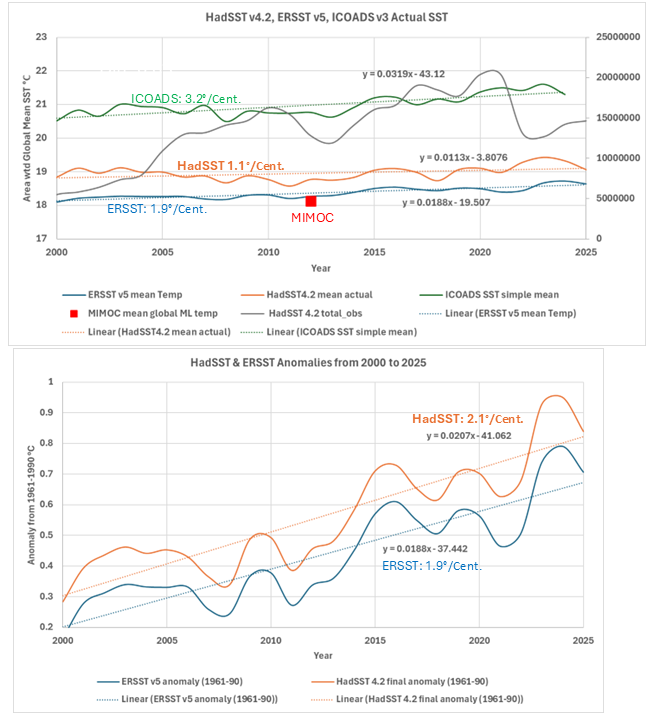
The gray line in the upper graph of figure 3 is the number of HadSST 4.2 ocean temperature observations, mostly in the mixed layer, in recent years. These observations are from ARGO float, ship, and buoy measurements (Kennedy J. et al., 2019). The other lines are global mean yearly mixed layer temperatures as estimated by various agencies. I should note that the NOAA ERSST grids (Huang et al., 2019) are fully infilled using extrapolation and assumptions about the SST under sea ice. HadSST is not (Kennedy et al., 2011) & (Kennedy et al., 2011b), and grid cells that have insufficient data are left null. This explains the difference between the HadSST and ERSST estimates in the upper graph in figure 3. The HadSST dataset has fewer populated cells in the colder polar water.

The bulk of the raw data used by the agencies in figure 3 comes from ICOADS, and ICOADS provides a simple mean shown as a green line in the upper plot (Freeman et al., 2017). Like HadSST, the differences in the ICOADS mean temperature are mostly a function of data coverage, gridding practices, corrections, and the amount of extrapolation and interpolation used in making the final global grids.

The mean temperature from NOAA MIMOC (Johnson et al., 2012) is from the ARGO era and plotted at 2012 arbitrarily. Since it is an average of many years it has no trend, but it is a complete grid like ERSST and plots close to ERSST. The point of figure 3 is that any EEI based on OHC is highly dependent upon the ocean dataset used. Figure 3 illustrates the variability in SST measurements (at about 20 cm depth) and the differences reflect uncertainties due to sampling error, measurement error, dataset construction choices, and measurement bias. The impact of long-term ocean oscillations, like the AMO, that demonstrate changes in shallow ocean thermal energy storage are also not considered. We must be careful when using OHC in any quantitative way without considering the data and methods used to compute it, especially over periods shorter than 100 years.

The lower graph in figure 3, shows the ERSST data in the upper graph converted into an anomaly from a 1961-1990 mean. It has the same slope or warming trend as the measurements in the upper graph. The final HadSST 4.2 anomaly shown in the lower graph has moved closer to ERSST, which is probably a function of making the anomaly from the 1961-1990 mean. After all the HadSST grid covers a different area than the ERSST grid. However, the HadSST slope has changed as a result of additional corrections performed after the anomaly was created. The new slope, which is closer to ERSST is solely a function of the corrections. This is not necessarily a bad thing, but it is notable that the SST warming trend can be changed so much as a function of data corrections.

Figure 4 shows ICOADS data coverage over time. Unlike ground weather stations, most of the ocean data is gathered by moving ships or drifting buoys and grid cell temperature is constructed over time using different sources and depth of measurement, although ERSST and HadSST try and correct the temperature for known biases and to a nominal 20 cm depth (Kennedy J. et al., 2019).

The ICOADS data are mostly uncorrected for bias and are not corrected for the measurements depth. The ICOADS measurement is described as the “near surface” measurement when multiple depths are available.

The notable thing about figure 4 is the lack of coverage in the Southern Ocean, the body of water connecting all oceans. Coverage in the Southern Pacific has decreased in recent years. Ocean temperature estimates below 2000 m are very sparse and while error has decreased in recent years it is still inadequate for estimating the Earth Energy Imbalance (Cohler et al., 2026). Neither the global mean mixed‑layer temperature nor its trend are known with sufficient accuracy.

The surface EEI varies at all time scales as shown in figure 5. As noted above, EEI is usually computed at the top of the atmosphere or TOA as the difference between the radiation entering the climate system and the radiation leaving it. But, because the TOA measurements are not accurate enough, the satellite measurements are adjusted to match ocean heat content changes. The OHC is affected by the radiation imbalance at the surface, which is separated from the TOA by a convection dominated troposphere where radiation energy transfer is a minor player. Thus, it makes sense to construct a “surface EEI” or more accurately a mean surface net radiation value.

The imbalance shown in figure 5 is the CERES net radiation (incoming-outgoing) hitting the surface, both longwave and short wave. Positive changes (up) mean more energy gained by the surface. It varies diurnally, with ENSO, the AMO, and all other ocean oscillations at periods of up to 60-70 years. The variations in surface EEI shown in the slide are computed from CERES EBAF (Loeb et al., 2018) data and are below the uncertainty in the satellite measurements. However, they are large compared to the AR6 calculated anthropogenic surface effect since 1750. Their estimate is 2.7 W/m² over 275 years and this graph shows differences of over 1.5 W/m² in less than 25 years. The Y axis values range from about 111 to 112 W/m², this is because most heat transfer from the surface is via latent heat due to evaporation and sensible heat transfer, both of which vary mostly due to wind speed.

The surface EEI also varies from one location to another as shown in figure 6. It is a map of the grid cell by grid cell surface EEI trends from 2001-2024. White is no change, red is a trend of +1 W/m² incoming over outgoing (that is energy gained by the surface) and blue is negative, that is more outgoing than incoming radiation. Figure 6 suggests that internal variability has a large effect on surface net radiation trends.

Flux balance

As discussed above, the energy fluxes at the 2D ocean/air interface must balance and the temperature profile inside and below the TSL changes to force them to balance. The TSL temperature profile changes throughout the day. Its heat capacity is limited (it’s only 0.1 to 0.5 mm thick), and it cannot send any net thermal energy downward because the net flux is to the surface and its viscosity prevents mixing. However, as Wong and Minnett show, it takes over the duty of sending energy into the atmosphere when it absorbs excess IR, which warms the atmosphere and has the effect of retaining more thermal energy (heat) in the mixed layer below.

Discussion

Longwave IR cannot meaningfully heat the mixed layer or deeper ocean because it is absorbed in the top 10–20 microns, which are colder than the water below and are continuously cooled by evaporation, sensible heat loss, and net longwave emission. The skin layer is too thin to store much heat, too cool to transmit heat downward, and too dominated by radiation and evaporative losses for IR to penetrate or accumulate. Only solar radiation significantly warms the bulk ocean.

The 340 W/m² of downwelling IR radiation shown in figure 2 is not an independent energy source, it is all recycled surface radiation except for the net flux out to space. The net outward radiation is the surface emission (398 W/m²) minus the downwelling (340 W/m²) or 58 W/m², which is much less than the incoming solar radiation (163 W/m²). The 340 W/m² is recycled many times (see Wim Röst’s figure 1 here).

Solar radiation directly increases mixed‑layer heat content, whereas GHG IR warms the ocean indirectly by reducing upward flux. These mechanisms are not equivalent, and their relative contributions depend on skin‑layer physics. The heat flow from the TSL is upward into the atmosphere; little can move downward, upgradient into the deeper ocean.

Due to the difficulty in measuring ocean surface temperatures in a consistent manner and the complexity of the constantly changing TSL temperature gradient, ocean heat content estimates are not precise enough to estimate the world ocean energy imbalance or even its trend over recent decades. The surface and upper ocean are warming, but the partitioning of heat between solar absorption and greenhouse‑gas‑mediated flux suppression remains uncertain because OHC datasets diverge and the skin‑layer physics complicates interpretation. The short time period since decent measurements of upper ocean heat content (2005 to the present) also complicates the issue. The AMO is 60-70 years, swamping our 21-year instrumental record, plus cloud cover is decreasing which increases insolation, bottom line, we do not know much.

In addition, as detailed by Judith Lean, Joanna Haigh, Hoyt and Schatten, and others, the impact of the Sun on climate is not a simple function of the amount of solar radiation that strikes Earth’s surface, there is much more involved (Lean, 2017), (Haigh, 2011), and (Hoyt & Schatten, 1997).

Download the bibliography here.